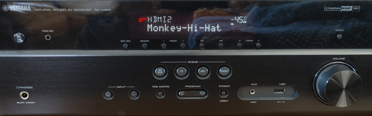
Monkey Hi Hat and Eyecandy Audio Textures

Understanding audio textures used by music visualizers.

This is the next installment in a series of articles about my Monkey Hi Hat music visualizer application, and the supporting libraries, applications, and content. You may wish to start with the earlier articles in this series:

• Introducing the Monkey Hi Hat Music Visualizer
• Monkey Hi Hat and the Eyecandy Library

The topic today is central to music visualization: understanding the audio data which is fed into the OpenGL shader programs and the formats available from this library.

Types of Audio Data

In the last article, I listed the three basic types of audio data:

• wave / PCM
• frequency
• volume

Wave audio data, also known as pulse-code-modulated or PCM, is best known as the data format used for compact disc recordings. It is literally a stream of 16-bit signed integers (short values in C#) representing the signal strength which moves speaker voice-coils (the magnet) in or out, via electrical pulses generated by an amplifer. Although, obviously, most modern amplifiers offer a wide variety of onboard signal processing, ranging from simple tone and equalizer adjustments to simulated surround sound on the more complex end of the spectrum, so “what comes out” is rarely directly matched to “what went in”.

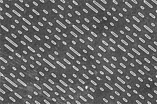
In fact, if you magnify the surface of a compact disc, you can literally see the “ones and zeroes” bit values that make up these signed short integers. The playback laser just reflects differently off these pits and peaks:

Naturally, modern, compressed, streaming music works very differently, but the resulting output is the same, as is the data generated by a computer’s “input device” audio-recording drivers. Note that CD audio and most other music sources are encoded in stereo. The library will downmix this to monoaural (single-channel) audio.

It’s tempting to think of wave audio as some sort of sine wave, but real-world audio is a wildly complex mixture of many different frequencies, and plotting the raw PCM data for anything but pure test tones is actually a random-looking jagged mess. This is where frequency data comes into play. A mathematical function called fast-Fourier transform (FFT) is used to identify the strength of the individual frequencies which are combined to produce a given PCM sample – low frequency bass sounds to high-frequency treble sounds. There are many ways to represent this data, but music viz typically uses either the decibel scale or a magnitude representation (strength relative to some baseline – zero, in this case).

The library also supports a kind of pseudo-frequency data which attempts to match the weird time-smoothed output from the browser-based WebAudio API. This is what you’ll probably use if you convert shaders from Shadertoy or VertexShaderArt.

Finally, there is volume, which is a surprisingly subjective thing. Most volume representations are “RMS volume”, which stands for root-mean-square, which is just a description of the math that is applied to a segment of PCM data. 300ms is commonly used because that’s how long it takes most people to register a change in volume. There are other algorithms out there, notably LUFS (Loudness Units relative to Full Scale) and the nearly-identical LKFS (Loudess K-weighted relative to Full Scale), but these are approximately the same as rating volume on the decibel scale, which is oriented to sound pressure rather than perceived loudness, which is what we want. Volume is an instantaneous or “point in time” value.

Some visualizers use PCM, but fewer than you might imagine. Frequency data is the most commonly used, and since the decibel scale produces a “stronger” signal across the frequency range, that representation seems to be preferred. Volume is often used as a sort of strength-multiplier (or, of course, any other effects you can imagine).

Even more information about audio data (such as calculations involving bit rates, sampling frequency, etc.) is available on the How It Works page of the Eyecandy wiki.

Audio Data as Shader Textures

As the previous article explained, for our purposes shader “textures” are really just two-dimensional data buffers, they aren’t graphical images in the sense normally implied by the word “texture”.

For wave and frequency data, the texture width corresponds to the number of audio samples captured at each interval. By default, the Eyecandy library generates 1024 samples, which equates to about 23ms of audio. (If you want to know where these numbers come from, refer to the wiki page linked in the last section.) That means most of these textures are 1024 data-elements wide (from now on, for simplicity I’ll just say “pixels” although the technically correct shader term would be “texels”).

The two exceptions are the volume data and the Shadertoy-oriented data. As explained in the last section, volume is a single point-in-time data element, so that texture is just one pixel wide. On the other hand, Shadertoy samples 1024 frequencies, but it only outputs the “lower” 512 frequencies, so that texture is only 512 pixels wide.

Technically speaking, PCM data is also point-in-time … it is the signal that should be sent to the speakers, 22,050 times per second per channel (for CD-audio-quality stereo data; other rates are possible and common). This means the width of the texture is technically a kind of history data – the audio signals over a 23ms timespan (at the default sampling values). But in practice, this is such a short period of time, the data still works well for code that wants to “show” the wave data which somewhat matches the music people are hearing.

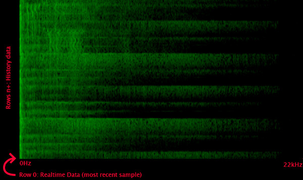
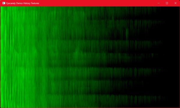
The note about PCM data notwithstanding, most of the Eyecandy audio texture options are also “history” textures. This defines the texture height. This means each time the audio capture engine has a new block of PCM data, the previous history data is shifted “upwards” in the bitmap by one row, and the new data is written into row zero. By default, the library stores 128 rows of history data. The amount of time represented by this data depends on the audio sampling rate. Using the library defaults, 128 rows is about three seconds (23ms x 128 = 2944ms).

This is what a decibel-scale frequency texture with history data looks like:

Currently, only the Shadertoy-style audio texture does not provide history data. Instead, row 0 is frequency data (WebAudio-style time-smoothed decibel-scale), and row 1 is PCM wave data.

In practice, the width doesn’t matter much because shaders normalize the data, meaning it is converted to a zero-to-one range. “0” is the “left edge” of the texture data, and “1” is the “right edge” regardless of whether it was originally generated as 1024 or 512 pixels. Shaders and GPUs are optimized to use floating point numbers, so you read (or “sample” in shader terminology) this data as 0.0 through 1.0. Requesting 0.5 is dead-center in the data, regardless of how many individual input pixels were originally used.

The only reason you might care about the original data resolution is when you want to pick out a specific frequency range. “Beat detection” is an important part of most music visualizers, and they tend to focus on the strongest signal, which will be in the bass range at or below about 100Hz. The math is explained in the wiki page mentioned earlier, but for 1024 samples, that means only the first 10 samples represent 100Hz or lower. Technically it’s the first 9.29, which in normalized shader-value terms would be 0.0929, but in practice it’s easiest to just use 0.0 through 0.1.

Finally, because shader textures really were originally intended to represent graphical images, the data is still stored as if it represented pixels. This means each input pixel has a certain bit-color-depth … 16 bits, 24 bits, 32 bits, or whatever. The data can also be defined as bytes, integers, floats, and sometimes other formats. Almost all GPUs and drivers always convert this to some standard internal representation. But in graphical terms, each pixel is normally described as RGB or more commonly RGBA format: red, green, and blue color channels, and an alpha transparency channel. This next point is very important:

Eyecandy usually stores data in the green channel.

There is at least one exception (the 4-channel history texture, which is discussed later) but this is particularly important if you’re converting shader code from some other system. For example, Shadertoy uses the red channel, and some Shadertoy code uses (u,v).x instead of (u,v).r which takes advantages of quirks of GLSL syntax (so-called “twizzling”).

The library exclusively uses normalized floats for audio texture data, so the data stored in each color channel is also in the 0.0 to 1.0 range.

Visualizing the Audio Textures

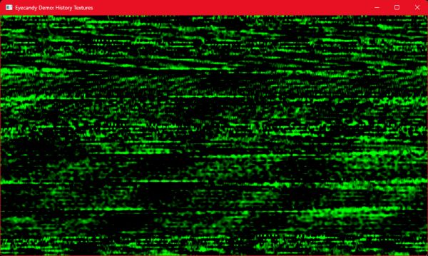
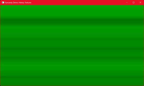
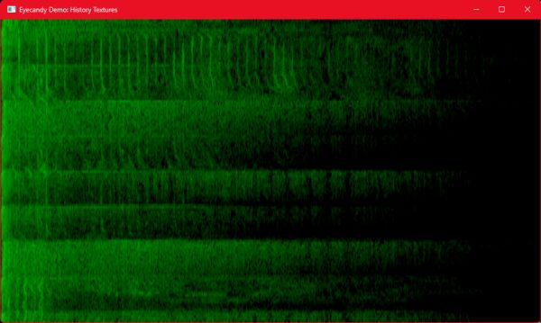
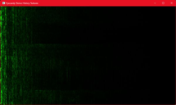
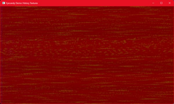
You’d think a series of articles about visualizations would have more pictures, but apparently that isn’t the case. Perhaps the most boring possible use of the Eyecandy audio textures is to treat them as literal images, and some of the demo program options do exactly that (the image in the previous section was produced this way).

First, we’ll take a look at the four “standard” audio representations, which is mostly what we’ve discussed so far. Because these are explained above, the images are presented without further discussion. The heading names are the Eyecandy class names that generate each texture.

AudioTextureWaveHistory

AudioTextureVolumeHistory

AudioTextureFrequencyDecibelHistory

AudioTextureFrequencyMagnitudeHistory

The library also offers three audio textures that warrant a bit of explanation.

AudioTexture4ChannelHistory

This one doesn’t lend itself well to direct visualization. Whereas most Eyecandy audio textures store data exclusively in the green channel, this class stores multiple types of data in each of the four RGBA channels. Red is volume, green is PCM wave data, blue is frequency using the magnitude scale, and alpha is frequency using the decibel scale.

AudioTextureWebAudioHistory

The WebAudio API defines a “time smoothing” algorithm applied to decibel-scale frequency data. The “realtime” sample is actually composed of 80% of the previous sample and only 20% of the new sample. If you compare this to true decibel-scale output, the result has a sort of smeared appearance. I’m not sure I really like this, particularly since it “drags out” artifacts after certain sharp sounds have actually ended, but the web-based visualizers all use it (they don’t really have any choice), so it’s important from the standpoint of conversion / compatibility.

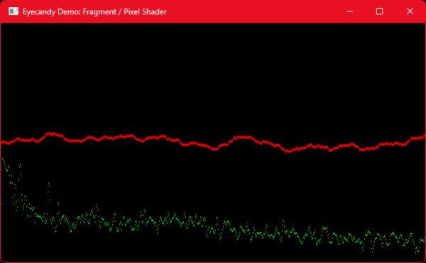
AudioTextureShadertoy

As noted earlier, the Shadertoy data isn’t a history texture. Instead, row 0 contains WebAudio-style decibel frequency data, and row 1 contains PCM wave data. As such, it doesn’t help to directly dump the texture to a window since you’d only see two faintly-pulsing lines, one on top of the other. Instead, this is a real Shadertoy shader that draws both data elements. The red line on top is PCM wave data, and the green output at the bottom is the frequency data.

Texel Center-Sampling Technique

There’s that word I said I wasn’t going to use: texel, which was coined from “texture pixel”. Unlike pixels in most traditional graphics file formats, where (5,8) refers to a specific individual RGBA pixel color and transparency, and you wouldn’t expect the neighboring pixels to matter at all, GPU textures use a normalized 0.0 to 1.0 range of floating point values. That means the best way to get the “true” value is to sample “the middle” of a texel.

Let’s consider the simple case of the Shadertoy data. Row 0 is PCM wave data, and row 1 is frequency data. But because the height is represented as 0.0 to 1.0, this means row 0 is most accurate with a y-value of 0.25, and row 1 is most accurate with a y-value of 0.75. There are two rows of discrete input data, so divide the 0.0 to 1.0 normalized range into two halves (0.0 to 0.5, and 0.5 to 1.0), then sample them using values from the center-value of each half: 0.25 and 0.75.

For audio viz, it’s rarely important to be that precise, but it’s useful to know.

Conclusion

Hopefully by this point you have a clear understanding of how Eyecandy represents audio data as shader texture buffers. There is a bit more detail in the repositories’ wikis on most of the topics covered here, if you wish to dig a little more deeply, but this should be enough to let you create audio visualization shaders.

The next installment will go into some of the implementation details of the library, then we’ll finally be ready to move on to the fun stuff: the Monkey Hi Hat music visualization program itself.