Monkey Hi Hat Getting Started Tutorial

Installing the program and writing a visualization shader.

Back in August of 2023, I published Introducing the Monkey Hi Hat Music Visualizer followed by several mostly-technical articles about the program and the underlying library. Version 2 added multi-pass rendering (described in this article), and version 3 had no article, but it involved a vast number of changes (which you can see in the wiki changelog). The most obvious version 3 improvement was the addition of post-processing effects. I have a lot of great new features and capabilities that I plan to release soon as version 4.

As I write this, the currently available version of Monkey Hi Hat (MHH) is 3.1.0, which you can find on the repository’s release page.

Edit: Version 4.0.0 was released February 1, 2024. A few related notes have been added to this article, mostly involving installation and configuration changes.

Even in the early days of the program’s life, it was apparent that it’s a little difficult to know where to start. It was initially necessary to follow many steps to install and use the program. These weren’t particularly complicated steps, but it looked like a lot of work and was probably off-putting to a lot of people. (The repository has a lot more views than downloads at this point, unfortunately.) These days the program features a Windows install script that makes the initial setup a lot easier, but one of my goals was to let people create new content, and that can still be hard to understand at first.

Note that the program still isn’t supported for Linux yet, but that is coming … I am actively documenting how to get it working on Debian under Windows Subsystem for Linux, aka WSL2. The Installation section below relates only to Windows, but if you’re reading this later on after I have Linux support again, the rest should apply to Linux, too, other than the specific format of path names, of course.

Installation

Edit: The Version 4.0.0 release includes a stand-alone install program which is much easier to use than the script-based installer described below. Just download it and run it and answer a few questions. This release also eliminates the need for the third-party audio loopback driver.

In the Assets section of the repository’s release page, you’ll see a link to install.ps1:

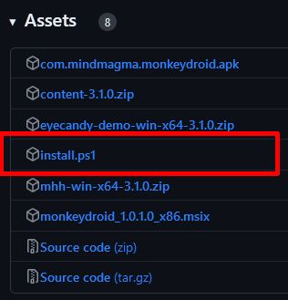
That script should be the only file you need to download to get the program working. You can just save it to your desktop, you won’t need it again after installation is complete. The installer is reasonably “smart” – it can handle partial installs, such as users who may already have some of the dependencies installed.

In theory, you should be able to right-click the file and choose Run with PowerShell:

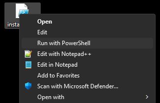
Unfortunately, by default Microsoft blocks PowerShell script execution. If you choose this option, Windows will load the script into an editor. I could go on a long rant about this (why not prompt, like UAC does? why offer a Run context menu option that doesn’t work?), but the fix is pretty easy:

• Open your Start menu and type Powershell to launch the scripting console
• Run this command: Set-ExecutionPolicy Unrestricted -Scope CurrentUser

Sigh. So much for making things easier on people. Thanks, Microsoft. After that, the Run menu command will work as expected. You’ll probably see a brief window flash – the script needs to bump itself up to admin rights to perform the installation. After that, it collects some information, shows you what it found, and asks a short series of questions. Generally you want to answer Y for Yes to everything. The last few relate to how you want to launch the application and are a matter of personal preference.

After you answer the questions, you’ll see a little banner appear across the top of your screen as several files are downloaded. The script will run the installers for the various dependencies, do some cleanup, and set up a default configuration for you.

If you didn’t already have the VB-Cable loopback audio driver installed (most people don’t), the script will offer to walk you through the configuration process for that driver. This is how the program “sees” the audio playing on your system, so it’s pretty important, and unfortunately it’s the only part that I can’t automate, because Microsoft doesn’t document how all of those settings are stored (and they’re too insanely complicated to safely reverse-engineer). Also, the program can’t tell which sound devices your computer has are the ones you really use. So you have to do that part by hand.

Just follow those directions, and if you have problems, similar directions are available in the repository’s wiki, which brings us to the next section…

Post-Installation Configuration

The wiki offers this page, which explains how to set up your computer’s audio after the installer runs. Once your audio is configured, you can do a test-run. That is also covered in the wiki in the Running for the First Time section on the wiki’s landing page.

Configuring your audio and doing a successful test run is very important, but if you want to create new content, you aren’t done yet.

The installer will automatically create a configuration file for you. On Windows you can find this at C:\Program Files\mhh\mhh.conf, and it’s just a text file that you can load into Notepad or any other plain text editor. When you first open it, you’ll see a whole bunch of settings. Near the top is a StartFullScreen setting which is true by default:

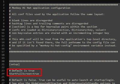
At a minimum, change that to false so that you can interactively work with the program from another window on the same computer. The Configuration Suggestions section is oriented to helping people who just want to run the program. If you’re planning to create your own content, there are some other config changes to consider.

The HideMousePointer setting is true by default, but it’s kind of annoying in windowed mode, so you may want to change that to false.

MHH can cache visualizations and effects as it runs, but if you’re actively working on them, it’s better to disable caching. You can do this from the command-line with the --nocache switch, but if you don’t want to have to remember to do this every time (or if you’re working on new content very frequently, as I do), it’s easier to permanently disable caching. Set the ShaderCacheSize, FXCacheSize, and LibraryCacheSize options to 0 to disable caching. Assuming your files are stored locally and you have a reasonably modern system, you probably won’t even notice the difference (caching makes a big difference if the files are stored on another computer or other network-based storage).

Finally, at the end of the file you will find a [windows] section, and at the end of that section are a bunch of directory-name entries created by the installer. As the names suggest, these tell the program where to find the content shown by the application:

Edit: The Version 4.0.0 release is able to update the path settings “in place” – they will no longer appear at the end of the configuration file as shown above.

“Out of the box” content comes from my Volt’s Laboratory repository, and the installer puts them on your system at C:\ProgramData\mhh-content. Generally speaking, you don’t want to mess with these since future updates will completely replace the contents of this directory.

For creating your own content, you want to create a whole separate directory structure, and those directories need to be added to the out-of-box directory names in the config file.

Create Your Content Directories

You can put your personal, custom content anywhere you like. This article will assume a top-level directory of C:\MyViz, but you can call it what you want, put it on other drives or a network share, nest it in your Documents directory, or whatever makes sense to you. After creating the top-level directory, create the five subdirectories shown below:

📂 C:\MyViz
      |--📂 fx
      |--📂 libraries
      |--📂 playlists
      |--📂 shaders
      +--📂 textures

Edit: The Version 4.0.0 release is able to update the path settings “in place” – they will no longer appear at the end of the configuration file as described in the rest of this section. Just find the applicable entries in the [windows] section of the config file.

Now go to the end of the configuration file and add those directories to the entries generated by the installer. The configuration most likely looks like this to start with:

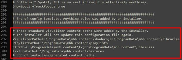
# These standard visualizer content paths were added by the installer.
# The installer will not update this configuration file again.
VisualizerPath=C:\ProgramData\mhh-content\shaders;C:\ProgramData\mhh-content\libraries
PlaylistPath=C:\ProgramData\mhh-content\playlists
FXPath=C:\ProgramData\mhh-content\fx;C:\ProgramData\mhh-content\libraries
TexturePath=C:\ProgramData\mhh-content\textures
# End of installer-generated content paths.

A semicolon ; is used to separate the directories. Notice that the libraries directory is referenced by both the FX and visualization directory lists (a list of directories or paths is called a “path specification”, commonly abbreviated to pathspec). Using the example, the config file pathspecs would change to this:

# These standard visualizer content paths were added by the installer.
# The installer will not update this configuration file again.
VisualizerPath=C:\ProgramData\mhh-content\shaders;C:\ProgramData\mhh-content\libraries;C:\MyViz\shaders;C:\MyViz\libraries
PlaylistPath=C:\ProgramData\mhh-content\playlists;C:\MyViz\playlists
FXPath=C:\ProgramData\mhh-content\fx;C:\ProgramData\mhh-content\libraries;C:\MyViz\fx;C:\MyViz\libraries
TexturePath=C:\ProgramData\mhh-content\textures;C:\MyViz\textures
# End of installer-generated content paths.

Basic Concepts

MHH runs OpenGL shaders which are graphics programs written in a language called GLSL. While a GLSL tutorial is far beyond the scope of anything I could cram into a blog article, you will need to know that language, but I will at least explain the code and commands used in the article. If you have any familiarity with C, it will be pretty easy to learn (though it is not identical by any means).

A single shader program is actually a combination of several smaller programs known as stages and MHH in particular only uses two of those: the vertex stage, and the fragment stage, or vert and frag as graphics programmers call them. These stages are usually also referred to as shaders, even though, technically, the shader is the combination of the two.

Although MHH is two-dimensional, OpenGL shader data is three-dimensional. The vertex stage sends the GPU a list of points in 3D space, and optionally other data like how to connect those points with lines, triangles, or a few other primitive shapes like line strips, triangle fans, and so on. Other shader stages convert that into screen output (the display area is usually called the viewport although I’ll probably screw up occasionally and write “screen”), and at the end of the process, the GPU knows which on-screen pixels represent “content” and which pixels are blank. It is the job of the fragment stage to color each of those pixels: the GPU will run the frag shader over and over again for each and every pixel that is part of the content described by the shader code in the vertex stage.

MHH visualizers can provide a program for both of these shader stages, or just one of the two. Currently the “out-of-box” shaders installed with MHH always uses just one or the other. Specifically, the vert-only shaders are mostly implementations adapted from the VertexShaderArt.com website, and the frag-only shaders are mostly implementations adapted from the Shadertoy.com website. Browse each site and you’ll quickly notice how they differ visually.

A vert-only shader is one which uses older-style OpenGL commands to draw very basic geometry, including individual points, possibly setting a larger-than-pixel point size, and the colors of the points, as well as simple shapes like lines or triangles. This tutorial won’t focus on those, but more information is available in the repository wiki.

A frag-only shader is what people usually think of if they have any experience with music visualization graphics like the famous MilkDrop. These can be challenging to write because the primary input data you have to work with is only the (x,y) coordinates of the pixel your program is supposed to color. That color is the output data. Virtually everything else has to be calculated – for every pixel.

Post-processing effects (FX) shaders work on the output of other primary visualization shaders, so they are always frag-only shaders.

Because a complete shader program is actually a combination of vert and frag shader stages, a vert-only shader still requires some frag code, but it’s a very simple pass-through that simply accepts the vert shader’s output color and itself outputs that color unchanged. Similarly, a frag-only shader has a reusable vert shader that simply provides coordinates for a shape that covers the entire display area, thereby ensuring the frag stage is called for every pixel. MHH is designed so that you only have to write the part you’re interested in (unless you really need to write both).

MHH coordinates all of this using different configuration or conf files. For example, the Volt’s Laboratory visualization called “acrylic” uses a file named acrylic.conf to describe the visualizer to MHH, and a GLSL frag stage program in a file named acrylic.frag. You’ll find both of them in C:\ProgramData\mhh-content\shaders on your local installation.

In addition to the basic inputs like (x,y) pixel coordinates, a shader can accept other data as inputs. There are two categories of inputs: varying and uniform inputs. The names refer to the nature of the data while a shader is generating a video frame. Varying data can change every time the program is called, whereas uniforms will not change for the duration of the frame being rendered. Generally speaking MHH shaders work with uniforms. Some are provided by MHH itself, like the number of seconds the shader has been running, the screen resolution, and other useful information. Others can be defined in the viz and fx config files. These can be fixed numbers, a random range of numbers, or external graphics files, known as textures.

The “primary” content for MHH is stored in the shaders directory for historical reasons, but they are referred to as visualizations, often shortened to viz. Special post-processing effects are referred to as FX and are stored in the fx directory. Reusable content is stored in the libraries directory and can be referenced by viz or FX shaders as needed.

Finally, you will probably want a text editor that understads the GLSL shader language. The popular Notepad++ can do this. If you are a programmer using Visual Studio, I recommend installing Daniel Scherzer’s excellent GLSL Language Integration extension.

Draw a Box

We’ll start with an extremely trivial example that just draws a white box on the screen. The .conf file describes the visualization to Monkey Hi Hat. Use your editor to create a text file called box.conf in your custom shaders directory (ie. C:\MyViz\shaders\box.conf). Copy this to the file and save it:

[shader]
Description=My First Shader
VertexSourceTypeName=VertexQuad
FragmentShaderFilename=box.frag

The Description line can be shown on-screen when MHH initially loads a visualization, and if you use my Monkey Droid remote-control application, it’ll be shown in that UI as well. Don’t worry about VertexSourceTypeName for now – suffice to say VertexQuad means that the vertex stage will describe a “quad” (rectangle) which covers the entire screen. Finally, FragmentShaderFilename is self-explanatory – the name of your frag program.

We’ll cover some of the other parts of a viz config later, but this wiki page documents all the available sections and settings. For now, let’s move on to the shader program itself.

Create another text file in your personal shaders directory called box.frag. Copy this to the file:

#version 450
precision highp float;

in vec2 fragCoord;
out vec4 fragColor;

void main()
{
}

This is the skeleton of the most basic-possible fragment shader.

#version 450 indicates OpenGL 4.5 is required. (The currently-available MHH and content uses 4.6, which is the newest [and final] version of OpenGL, but Linux MESA drivers only support 4.5, and 4.6 doesn’t have any features needed by MHH, so going forward MHH will only require the OpenGL 4.5 core API level.) The #version directive must always be the first line in the shader (verts and frags).

The second line, precision highp float, just tells the GPU to use high-precision numbers. Some older, cheaper GPUs don’t support this, but you probably wouldn’t be able to run MHH visualizations on those anyway.

The next two lines define inputs and outputs. The vec2 and vec4 data types are two- and four-component vector variables, respectively. This means your program can refer to individual x and y values stored in the fragCoord input data: fragCoord.x and fragCoord.y, which represent the (x,y) coordinates the fragment program is supposed to generate. The four components for fragColor are xyzw, or alternately rgba, so to read or change the red channel of the output color, you would reference fragColor.r.

The void main() section is the program entry point. You can define functions and variables outside of this, but they generally must be declared above the main() function, otherwise most driver’s compilers will refuse to compile the shader programs. (These source code text files are read into memory and passed to the graphics driver in real time, as the program runs. Shaders are normally not pre-compiled since every vendor’s drivers handle compilation differently, so you can’t know ahead of time what your users will have installed.)

The OpenGL coordinate system is normalized which just means all values are in the zero-to-one range. Generally speaking, most shader data uses the float data type. GPUs are highly optimized for working with fractional floating-point numbers. Thus, the (x,y) coordinates across the whole viewport ranges from (0, 0) to (1, 1). The exact center of the viewport (regardless of resolution or aspect ratio) is always (0.5, 0.5). Coordinate (0, 0) is the bottom left, and (1, 1) is the top right (exactly like the positive quadrant of a Cartesian grid in the geometry lessons you probably had in school).

In fact, just about everything is normalized, even color data. The RGB value for pure white is (1,1,1), which raises an important point: the GLSL language is very picky about how you represent numbers. Since vectors like vec2 and vec4 store floating-point values, you have to explicitly write your code to use decimal values:

vec3 white;
white.r = 1.0;  // compiler recognizes "1.0" as floating-point
white.g = 1.0;
white.b = 1.0;

This will not compile:

vec3 white;
white.r = 1;  // error: compiler thinks "1" is an integer
white.g = 1;
white.b = 1;

Update box.frag with the code to draw a white box at the center of the screen:

#version 450
precision highp float;

in vec2 fragCoord;
out vec4 fragColor;

void main()
{
    fragColor = vec4(0.0);

    if(fragCoord.y >= 0.25 && fragCoord.y <= 0.75)
    {
        if(fragCoord.x >= 0.25 && fragCoord.x <= 0.75)
        {
            fragColor = vec4(1.0, 1.0, 1.0, 1.0);
        }
    }
}

First, we initialize the output color to black using a single input value to the vec4 constructor – all four components, the RGB values and the alpha value, are set to zero, expressed as a floating-point number, 0.0. (It is a strange quirk of GLSL that you can actually specify an integer here, even though it’ll be stored as floating point, but I don’t like to do that because they aren’t freely interchangeable anywhere else.)

Next we inspect the (x,y) coordinates to see if they’re within the center 50% of the screen area vertically and horizontally (remember that fragCoord holds normalized values, 0.0 through 1.0). If both of those are true, we change the output color to white by specifying all four components of the vec4 constructor.

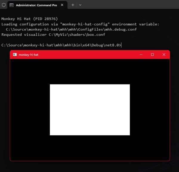
Save these changes and run Monkey Hi Hat. When the idle shader is visible, open another console window, change to the MHH program directory, and issue the command to load your new visualization:

mhh --load box

If everything is set up correctly, you’ll see the results of your program:

Use a Uniform Input

MHH exposes a number of useful values that a shader can use. They’re all documented here in the wiki, but in this case we’ll use randomrun which is a normalized (0.0 to 1.0) random number that is generated each time a shader is loaded. Here is the new code for box.frag:

#version 450
precision highp float;

in vec2 fragCoord;
uniform float randomrun;
out vec4 fragColor;

void main()
{
    fragColor = vec4(0.0);

    float r = clamp(randomrun * 0.5, 0.05, 0.45);

    if(fragCoord.y >= r && fragCoord.y <= (1.0 - r))
    {
        if(fragCoord.x >= r && fragCoord.x <= (1.0 - r))
        {
            fragColor = vec4(1.0, 1.0, 1.0, 1.0);
        }
    }
}

In this version, line 5 declares a uniform input that is a normalized float data type named randomrun. The MHH program tries to pass this value (and the other uniforms listed in the wiki) regardless of whether the shader actually uses it. Now each time you load the box visualization, the size of the white box will change. In reality we’re working from the center of the viewport, which is halfway to 1.0, so we multiply randomrange by half. We also use the clamp function to ensure the result is never less than 0.05 and never more than 0.45, which ensures the box is always visible but never covers the entire viewport.

Load an Image File

That box is pretty dull, so let’s try something more interesting. Find a graphics file and drop it into your textures directory. Generally speaking, you should avoid very large files, both in raw size and in resolution dimensions. GPUs are extremely good at scaling images and you’d be quite surprised at the picture quality you can get from even a relatively small input (in modern terms) such as 1024x1024.

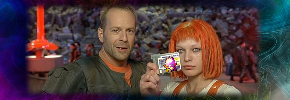
For the article, my example uses a JPEG named Queen Cersei Lannister.jpg, which features one of our food-obsessed dogs. As you can see, spaces are fine in the filename. Add the [textures] section to your box.conf viz config file as shown below, but replace the filename with whatever you copied to your textures directory:

[shader]
Description=My First Shader
VertexSourceTypeName=VertexQuad
FragmentShaderFilename=box.frag

[textures]
tutorial : Queen Cersei Lannister.jpg

The tutorial portion is the name of the uniform that MHH will use to provide a copy of the image to the shader at runtime. This is a good time to point out that GLSL (like the C language) is case-sensitive.

Update the code in the box.frag shader as follows:

#version 450
precision highp float;

in vec2 fragCoord;
uniform sampler2D tutorial;
out vec4 fragColor;

void main()
{
    vec3 image = texture(tutorial, fragCoord).rgb;
    fragColor = vec4(image, 1.0);
}

When you tell MHH to load this visualization, you should see the image you chose, scaled (and probably distorted) to match whatever dimensions your viewport happens to be using. You can resize the window and the image will adjust to keep the viewport filled with the image.

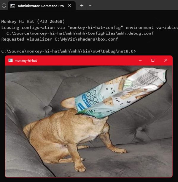
This code shows a couple of important things. First, obviously, is that the texture data is a special sampler2D data type, and of course the uniform name tutorial matches the name we assigned in the viz config file.

It uses the GLSL texture command to read (or sample in shader terminology) a portion of the graphics buffer which stores the image. The command returns a vec4 (RGBA data), but in this case we’re only storing the RGB channels into a vec3 variable named image – notice the .rgb at the end of the command. The two arguments to this command are the reference to the texture itself (which we’ve stored in the tutorial uniform), and the normalized coordinates to be sampled.

Using normalized coordinates for the texture implies that the image stored in the texture buffer, regardless of the original file’s resolution or other details like the aspect ratio, is also represented by a range of floating-point values from (0.0, 0.0) through (1.0, 1.0).

This is why we can specify fragCoord as the second argument, even though fragCoord is one of the shader’s input values that describes which pixel to output. The rendering viewport might be 1920 x 1080 but the texture image might only be 1024 x 768 – not even the same aspect. But thanks to normalized coordinates, 0.5 is always going to represent the center of both. Because the shader program is executed with fragCoord values ranging from (0.0, 0.0) to (1.0, 1.0), telling the texture command “give me the texture color at position (0.25, 0.25)” is always going to be a point from the lower left quarter of the image, and outputting it for that same coordinate will always display in the lower left quarter of the viewport.

This is why it’s called a sampler and we say we are sampling the texture: the GPU is able to very, very quickly “interpolate” the colors – sort of like resizing the image on the fly, scaling it up or down as needed. In fact, we don’t refer to “pixels” when we’re sampling a texture this way, we refer to texels so that it’s clear we’re talking about something other than the original raw image data.

To put it another way, if the viewport is 1920 x 1080, rendering a fragCoord of (0.3, 0.3) means we’re calculating the final displayed color of the pixel at (576, 324), but if we’re sampling (0.3, 0.3) from a 1024 x 768 texture, we’re reading interpolated texel color data from position (307.2, 230.4): not exactly one specific pixel from the source image, but a value that is a mix of the pixels nearest to the requested location.

Aspect Ratio Correction

You may have suspected that the picture of my dog is “squished” as my wife described it. The program simply spits out the fragCoord-based texels with no consideration for how it looks. Specifically, it ignores the original texture’s aspect ratio, which is simply the relationship between the original image file’s width and height. There is a simple calculation to scale an image to a target viewport.

Even though this section is going to show you how to address this, shader programmers actually don’t commonly worry about aspect ratio in most texture scenarios, because input textures are rarely directly used as stand-alone images. They are more often used to provide abstract data (such as pseudo-random noise, or in the case of MHH, a representation of audio), or “texturing” via small tiling images used to simulate a material or surface like cloth, wood, or stone. But correcting for aspect ratio is easy, it’s a good example of the sorts of problems you need to solve when you write a shader, and it gives us an excuse to discuss uv which is another shader programming convention that you’ll encounter frequently.

So, while our little dog may be food-obsessed, she isn’t actually fat (or squished) … let’s do something about that aspect ratio.

The GLSL command textureSize returns the source image resolution. The question then becomes what to do with the rendered pixels that are not covered by the image? We are going to adaptively scale by the largest dimension, whether it is the width or the height, and any “unused” pixels will simply be rendered in black. Alternately, you could calculate other display strategies, such as filling the screen regardless of clipping, for example, or rendering a faded and blurred version of the edges of the image in the unused areas, as some image viewing programs do. It all depends on what you’re trying to achieve. But for now, we’ll keep it simple.

Here is the new box.frag shader:

#version 450
precision highp float;

in vec2 fragCoord;
uniform vec2 resolution;
uniform sampler2D tutorial;
out vec4 fragColor;

void main()
{
    vec2 texRes = vec2(textureSize(tutorial, 0));
    vec2 scaling = resolution / texRes;

    vec2 uv = fragCoord * resolution;

    uv -= 0.5 * texRes * max(vec2(scaling.x - scaling.y, scaling.y - scaling.x), 0.0);

    uv /= texRes * min(scaling.x, scaling.y);
    
    fragColor = (uv == fract(uv))
        ? texture(tutorial, uv)
        : vec4(0.0);
}

When you run this version, no matter what dimensions you make the window, the image will be shown at the correct aspect ratio:

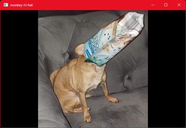
Notice that we’ve declared another input uniform provided by MHH: resolution is a vec2 that represents the (x,y) size of the viewport.

The textureSize command accepts two arguments – the sampler uniform, and the level of detail or LOD index. We aren’t using LOD (it’s more useful in 3D applications), so we simply set that to zero to use the original image (MHH doesn’t configure the textures to generate LOD, so they aren’t available even if you wanted to use them). Notice that we don’t directly use the return value from textureSize, but instead we wrap it with a vec2 constructor. This is because we want floating point (x,y) values, but textureSize returns integers using the ivec2 data type.

Next, we create a pair of scaling factors. Notice that scaling is a vec2 meaning it provides scaling.x and scaling.y elements. It is set to the viewport resolution divided by the texture resolution. GLSL allows us to perform mathematical operations on variables of the same type without having to reference each individual component. This is equivalent to separately writing:

vec2 scaling;
scaling.x = resolution.x / texRes.x;
scaling.y = resolution.y / texRes.y;

We’ll get back to the scaling factor in a moment.

We use the same feature to multiply two other vec2 values: the fragCoord value, which is the normalized 0.0 to 1.0 (x,y) coordinates of the pixel to render, by the viewport resolution, which is the true pixel size of the rendering window’s drawing surface. The result is stored in the vec2 variable named uv. This result the denormalized (x,y) coordinate – the actual discrete pixel x and y values. In other words, if the resolution is 800 x 600, and fragCoord is (0.5, 0.5), that yields the pixel coordinate (400, 300) at the center of the screen. Why uv? This is another convention in the graphics programming world. Any variable named “uv” is understood to (usually) hold some alternate representation of (x,y) coordinates. To confuse matters, in some systems like Shadertoy, both fragCoord and uv generally mean the opposite of what they mean in pure OpenGL: the Shadertoy fragCoord input is a denormalized pixel coordinate, and uv is commonly assigned to the normalized equivalent. For now, the important point is to remember that when you see uv you’re probably looking at some sort of coordinate data.

Next is a calculation which basically offsets the center of the image from the center of the screen. You might wish to draw this out on a scrap of paper to understand how and why it works. (It should go without saying that the GLSL max command simply returns the larger of two values.)

There is no “right” or “wrong” resolution or aspect ratio, and in this age of portrait-mode mobile phone pictures and videos, we can’t even say that wider images are more common than taller images. Much of the time, shader programming is about taking mathematical shortcuts. In this case, we calculated two scaling factors in one shot, which accomodates both aspect ratio scenarios – images that are either wider or taller. It’s easier to understand with hard numbers.

The picture of my dog happens to have a resolution of 495 x 529. These odd dimensions are because I clipped it from a much larger source image without worrying about the specific dimensions. Let’s assume for a moment that our output viewport is 800 x 600. This yields a horizontal scaling factor of 800 / 495, or 1.61, and a vertical scaling factor of 600 / 529, or 1.13. These are calculated and stored in scaling.xy by the single resolution / texRes operation. The smaller of these two, which is 1.13 on the vertical axis, tells us which dimension is larger. To fit the entire image into the viewport, we’ll scale the texture by that factor. This fits the largest dimension into the viewport, and keeps the other dimension scaled by the same factor so that the image looks correct.

So the next line uses the same vector math support to multiply the original texture resolution by the smallest viewport scaling factor, and the phyiscal coordinates offset from the center are divided by this value, which turns uv back into normalized (0.0 to 1.0) coordinates, which will be required by the texture sampling command.

Finally, a ternary assignment is used to either output the sampled texel at the uv coordinate, or a black pixel (RGBA all set to zero). A ternary assignment is shorthand for an if/else conditional statement block. The syntax is variable = (conditional) ? true_value : false_value and the long form would be written this way:

if(uv == fract(uv))
{
    fragColor = texture(tutorial, uv);
}
else
{
    fragColor = vec4(0.0);
}

The GLSL command fract returns the fractional portion of a number. That conditional is just a trick that is equivalent to uv < 1.0 and is another example of the sort of oddities you will see “in the wild” on sites like Shadertoy. In fact, this example was simplified and translated for readability from this Shadertoy program, believe it or not (click the link and compare the code).

A few other things you could do with very minor changes to this code (which are mentioned as comments in the Shadertoy original linked above):

• Always scale by height, even if the width is larger: uv /= texRes * scaling.y;
• Always scale by width, regardless of height: uv /= texRes * scaling.x;
• Half-scale the image by adding a line before fragColor is set: uv *= 2.0;

But What About Music?

The point of MHH, of course, is music visualization. Earlier we mentioned textures can be used for abstract data sharing, rather than anything we’d consider an image. Audio data is available in several formats, all of which are discussed in my September 2023 article, Monkey Hi Hat and Eyecandy Audio Textures. Decibel-scale frequency data is probably the most useful representation, so we’ll use the eyecandy AudioTextureFrequencyDecibelHistory which the Understanding Audio Textures page of the MHH wiki tells us is available as a uniform named eyecandyFreqDB.

First we’ll add an [audiotextures] section to box.conf to tell MHH that the visualizer needs that data. It’s as simple as listing the uniform name under the section tag:

[shader]
Description=My First Shader
VertexSourceTypeName=VertexQuad
FragmentShaderFilename=box.frag

[textures]
tutorial : Queen Cersei Lannister.jpg

[audiotextures]
eyecandyFreqDB

Now let’s modify the frag shader to use this data:

#version 450
precision highp float;

in vec2 fragCoord;
uniform vec2 resolution;
uniform sampler2D tutorial;
uniform sampler2D eyecandyFreqDB;
out vec4 fragColor;

void main()
{
    vec2 texRes = vec2(textureSize(tutorial, 0));
    vec2 scaling = resolution / texRes;

    vec2 uv = fragCoord * resolution;

    uv -= 0.5 * texRes * max(vec2(scaling.x - scaling.y, scaling.y - scaling.x), 0.0);

    uv /= texRes * min(scaling.x, scaling.y);
  
    float beat = texelFetch(eyecandyFreqDB, ivec2(1, 0), 0).g;
    uv *= 1.5 + beat;

    fragColor = (uv == fract(uv))
        ? texture(tutorial, uv)
        : vec4(0.0);
}

There isn’t anything I could show you as a still-frame image, but if you play some music and run this, the image is slightly scaled according to the beat. It won’t win any awards, but it demonstrates the technique.

Instead of sampling the data with the texture command, this example uses a command called texelFetch. The input is, again, a sampler2D texture buffer, but the coordinate is a denormalized integer-based ivec2 data type. The output is a specific pixel from the original texture – interpolation is not used. In this case we’re reading the (x,y) coordinate (1, 0), meaning the second column of the first row of pixel data. The third argument is level of detail (LOD) like we mentioned for the textureSize command, and again we aren’t using it so we pass a zero. Finally, we only retrieve the green channel (.g) since that is where eyecandy stores audio data in most of these textures.

FX: Post-Processing Effects

This article is already running very long, so I’m going to speed things up a bit. I wanted to quickly walk through the creation of an FX shader. The basic concepts are similar: a config file describes the FX to MHH, and a frag file contains the code. However, an FX uses the output of a primary visualization shader (like our simple “box” example) as the input to the FX shader. Whatever the viz generates is stored into a texture, and that is handed off as a sampler2D uniform to the FX shader. This is the most basic example of multi-pass rendering (if you like technical details, check out my article Monkey Hi Hat OpenGL Multi-Pass Rendering). This makes the config file a little more complicated because many FX use several passes.

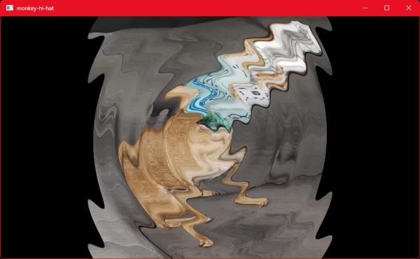
We’re going to create a simple spiral displacement effect that is similar to the Swirly FX included with an MHH install.

Go to your custom content fx directory and create sprial.conf (ie. C:\MyViz\fx\spiral.conf) and save this in the file:

[fx]
Description=My First FX

[multipass]
1 0 spiral.frag

Like a visualizer config, Description can be shown on-screen when the FX is loaded. (Currently the Monkey Droid remote-control program doesn’t support FX, but eventually it will also be visible in that UI.) There are many other options which you can read about here in the MHH wiki.

The [multipass] section defines output buffers and input textures for shader passes. The first column lists the output buffer used for each pass. These are zero-based, but the visualizer being modified by the FX is always buffer zero, so an FX always starts by outputting to buffer 1. The second column lists which buffers are used as input textures. This example uses buffer 0 as the input, which means the visualizer’s final output frame is provided as an input texture to this FX shader. The uniform names reflect these buffer numbers, so spiral.frag should expect to receive a sampler2D named input0.

In your fx directory, create spiral.frag with this content:

#version 450
precision highp float;

in vec2 fragCoord;
uniform vec2 resolution;
uniform float time;
uniform sampler2D input0;
out vec4 fragColor;

float time_frequency = 1.0;       // change over time (hertz)
float spiral_frequency = 10.0;    // vertical ripple peaks
float displacement_amount = 0.02; // how much the spiral twists

#define fragCoord (fragCoord * resolution)

const float PI = 3.14159265359;
const float TWO_PI = 6.28318530718;
const float PI_OVER_TWO = 1.57079632679;

void main()
{
    vec2 uv_screen = fragCoord / resolution.xy;
    vec2 uv = (fragCoord - resolution.xy * 0.5) / resolution.y;
    
    vec2 uv_spiral = sin(vec2(-TWO_PI * time * time_frequency +         //causes change over time
                              atan(uv.x, uv.y) +                        //creates the spiral
                              length(uv) * spiral_frequency * TWO_PI,   //creates the ripples
                              0.));

    fragColor = vec4(texture(input0, uv_screen + uv_spiral * displacement_amount));
}

By now, you should be able to recognize most of this. We’re declaring another MHH-provided uniform called time which is the number of seconds elapsed since the shader started running. (In this case, that refers to the FX shader only; the visualizer has a separate time uniform that is only available to that program.)

Since this code is based on something from Shadertoy, it assumes the “backwards” interpretation of fragCoord, so we add a #define macro in line 14. Anywhere the program refers to fragCoord, the calculation (fragCoord * resolution) is applied, which gives us the Shadertoy-style denormalized interpretation of fragCoord. Ironically, this is often to support a uv calculation which turns right around and normalizes that value. But such tricks do make porting easier, and most compilers will optimize that anyway, so it isn’t worth worrying about too much.

You can load a visualizer plus a specific FX with one command:

mhh --load box spiral

For this section, I reverted box.frag to the non-audio version. The result is a moving spiral displacement of the correctly-scaled target image:

Custom Uniform Values

One final technique I want to demonstrate is modifying uniforms from config files.

Change the three float variables in spiral.frag to uniforms:

uniform float time_frequency = 1.0;       // change over time (hertz)
uniform float spiral_frequency = 10.0;    // vertical ripple peaks
uniform float displacement_amount = 0.02; // how much the spiral twists

As you can see, these uniforms have a default value. If the program does not provide a value, the defaults will be used.

MHH doesn’t know about these particular uniforms, so we can control them from the FX config file. Add this [uniforms] section to your FX spiral.conf:

[fx]
Description=My First FX

[multipass]
1 0 spiral.frag

[uniforms]
time_frequency = 4.0

Now if you execute the visualizer and the FX, the ripples move much more quickly.

You can also randomize that value. Change the line in the configuration file to this:

time_frequency = 0.25 : 4.0

Now when the FX is started the uniform will be set to some random value between those two numbers (inclusive).

A visualizer config can control uniforms in its own shader programs in the same way. But a visualizer can also control the uniforms for a specific FX when it is applied to that visualizer. Go back to your box.conf file and add this to the end:

[fx-uniforms:spiral]
spiral_frequency = 5.0 : 20.0
displacement_amount = 0.01 : 0.10

Now when you run the visualizer and the FX, everything is randomized. The FX config randomizes time_frequency, but the visualizer config randomizes spiral_frequency and displacement_amount.

Note that if a uniform is defined in both config files, the visualizer will take precedence. This is interesting because an FX can provide some randomized values for visualizers which are “unaware” of the FX, but visualizers with special needs (or that have problems with certain FX values) can override those settings. This also allows FX to expose “controls” to the visualizers. For example, the first pass shader in Volt’s Laboratory FX meltdown exposes an option_mode uniform that lets a visualizer “activate” one of four color-matching calculations.

Conclusion

I realize this “simple” tutorial ran pretty long, but hopefully it will help people get their bearings with Monkey Hi Hat. Visualizers and FX can do a lot more than is covered here, and we haven’t scratched the surface of other Monkey Hi Hat features like library and crossfade support. If you use the program, please drop me a note to tell me what you think, and as always, I’m interested in questions, ideas, pull requests, new content, or whatever else comes to mind.